Getting Started

Connecting to LeapYear and Exploring

The first step to using LeapYear’s data security platform for analysis is getting connected. To get started, we’ll import the Client object from the leapyear python library and connect to the LeapYear server using our user credentials.

Credentials used for this tutorial:

>>> url = 'http://localhost:{}'.format(os.environ.get('LY_PORT', 4401))
>>> username = 'tutorial_user'
>>> password = 'abcdefghiXYZ1!'

Import the Client object:

>>> from leapyear import Client

Create a connection:

>>> client = Client(url, username, password)
>>> client.connected
True
>>> client.close()
>>> client.connected
False

Alternatively, Client is also a context manager, so the connection is automatically closed at the end of a with block:

>>> with Client(url, username, password) as client:
...     # carry out computations with connection to LeapYear
...     client.connected
True
>>> client.connected
False

Databases, Tables and Columns

Once we’ve obtained a connection to LeapYear, we can look through the databases and tables that are available for data analysis:

>>> client = Client(url, username, password)

Examine databases available to the user:

>>> client.databases.keys()
dict_keys(['tutorial'])
>>> tutorial_db = client.databases['tutorial']
>>> tutorial_db
<Database tutorial>

Examine tables within the database tutorial:

>>> sorted(tutorial_db.tables.keys())  
['classification',
 'regression1',
 'regression2',
 'twoclass']
>>> example1 = tutorial_db.tables['regression1']
>>> example1
<Table tutorial.regression1>

Examine the columns on table tutorial_db.regression1:

>>> example1.columns  
{'x0': <TableColumn tutorial.regression1.x0: type='REAL' bounds=(-4.0, 4.0)     nullable=False>,
 'x1': <TableColumn tutorial.regression1.x1: type='REAL' bounds=(-4.0, 4.0)     nullable=False>,
 'x2': <TableColumn tutorial.regression1.x2: type='REAL' bounds=(-4.0, 4.0)     nullable=False>,
 'y':  <TableColumn tutorial.regression1.y:  type='REAL' bounds=(-400.0, 400.0) nullable=False>}

Column Types

TableColumn objects include their type, bounds, and nullability.

>>> col_x0 = example1.columns['x0']
>>> col_x0.type
<ColumnType.REAL: 'REAL'>
>>> col_x0.bounds
(-4.0, 4.0)
>>> col_x0.nullable
False

The possible types are: BOOL, INT, REAL, FACTOR, DATE, TEXT, and DATETIME.

INT, REAL, DATE, and DATETIME have publicly available bounds, representing the lower and upper limits of the data in the column. FACTOR also has bounds, representing the set of strings available in the column. BOOL and TEXT columns have no bounds.

The DataSet Class

Once we’ve established a connection to the LeapYear server using the Client class, we can import the DataSet to access and analyze tables.

>>> from leapyear import DataSet

We can access tables, either using the client interface as above:

>>> ds_example1 = DataSet.from_table(example1)

or by directly referencing the table by name:

>>> ds_example1 = DataSet.from_table('tutorial.regression1')

The DataSet class is the primary way of interacting with data in the LeapYear system. A DataSet is associated with collection of Attributes, which can be used to compute statistics. The DataSet class allows the user to manipulate and analyze the attributes of a data source using a variety of relational operations such as column selection, row selection based on conditions, unions, joins, etc.

An instance of the Attribute class represents either an individual named column in the DataSet or a transformation of one or several of such columns via supported operations. Attributes also have types, which can be inspected the same as the types in a DataSet schema. Attributes can be manipulated using most built in Python operations, such as +, *, and abs.

>>> ds_example1.schema  
Schema([('x0', AttributeType(name='REAL', nullable=False, domain=(-4, 4))),
        ('x1', AttributeType(name='REAL', nullable=False, domain=(-4, 4))),
        ('x2', AttributeType(name='REAL', nullable=False, domain=(-4, 4))),
        ('y',  AttributeType(name='REAL', nullable=False, domain=(-400, 400)))])
>>> ds_example1.schema['x0']
AttributeType(name='REAL', nullable=False, domain=(-4, 4))
>>> ds_example1.schema['x0'].name
'REAL'
>>> ds_example1.schema['x0'].nullable
False
>>> ds_example1.schema['x0'].domain
(-4.0, 4.0)
>>> attr_x0 = ds_example1['x0']
>>> attr_x0
<Attribute: x0>
>>> attr_x0 + 4
<Attribute: x0 + 4>
>>> attr_x0.type
AttributeType(name='REAL', nullable=False, domain=(-4, 4))
>>> attr_x0.type.name
'REAL'
>>> attr_x0.type.nullable
False
>>> attr_x0.type.domain
(-4.0, 4.0)

In the following example, we’ll take a few attributes from the table tutorial.regression1, adding one to the x1 attribute and multiplying x2 by three. The bounds are altered to reflect the change.

>>> ds1 = ds_example1.map_attributes(
...     {'x1': lambda att: att + 1.0, 'x2': lambda att: att * 3.0}
... )
>>> ds1.schema  
Schema([('x0', AttributeType(name='REAL', nullable=False, domain=(-4, 4))),
        ('x1', AttributeType(name='REAL', nullable=False, domain=(-3, 5))),
        ('x2', AttributeType(name='REAL', nullable=False, domain=(-12, 12))),
        ('y',  AttributeType(name='REAL', nullable=False, domain=(-400, 400)))])

We can use DataSet to filter the data to examine subsets of the data, e.g. by applying predicates to the data:

>>> ds2 = ds_example1.where(ds_example1['x1'] > 1)
>>> ds2.schema  
Schema([('x0', AttributeType(name='REAL', nullable=False, domain=(-4, 4))),
        ('x1', AttributeType(name='REAL', nullable=False, domain=(1, 4))),
        ('x2', AttributeType(name='REAL', nullable=False, domain=(-4, 4))),
        ('y',  AttributeType(name='REAL', nullable=False, domain=(-400, 400)))])

Data Analysis

Statistics

The LeapYear system is designed to allow access to various statistical functions and develop machine learning models based on data in DataSet. The analytics function is not executed until the run() method is called on it. This allows inspection of the overall workflow and early reporting of errors. All analysis functions are located in the leapyear.analytics module.

>>> import leapyear.analytics as analytics

Many common statistics functions are available including:

• count()

• count_distinct()

• median()

• min()

• max()

• mean()

• sum()

• variance()

• histogram()

Next is an example of obtaining simple statistics from the dataset:

>>> mean_analysis = analytics.mean('x0', ds_example1)
>>> mean_analysis.run()
0.039159280186637294
>>> variance_analysis = analytics.variance('x0', ds_example1)
>>> variance_analysis.run()
1.0477940098374177
>>> quantile_analysis = analytics.quantile(0.25, 'x0', ds_example1)
>>> quantile_analysis.run()
-0.6575000000000001

By combining statistics with the ability to transform and filter data, we can look at various statistics associated to subsets of the data:

>>> analytics.mean('x0', ds_example1).run()
0.039159280186637294
>>> ds2 = ds_example1.where(ds_example1['x1'] > 1)
>>> analytics.mean('x0', ds2).run()
0.14454229785771325

Machine Learning

The leapyear.analytics module also supports various machine learning (ML) models, including

• regression-based models (linear, logistic, generalized),

• tree-based models (random forests for classification and regression tasks),

• unsupervised models (e.g. K-means, PCA),

• the ability do optimize model hyperparemeters via search with cross-validation, and

• the ability to evaluate model performance based on a variety of common validation metrics.

In this section we will share some examples of the machine learning tools provided by the LeapYear system.

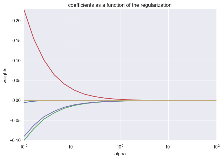
The Effect of L2 Regularization on Model Coefficients

The following example code shows a common theoretical result from ML: as the L2 regularization parameter alpha increases, we see the coefficients of the model gradually approach zero. This is depicted in the graph generated below:

>>> n_alphas = 20
>>> alphas = np.logspace(-2,2, n_alphas)
>>>
>>> # example3 has 0 and 1 in the y column. Here, we convert 1 to True and 0 to False
>>> ds_example3 = DataSet\
...    .from_table('tutorial.classification')\
...    .map_attribute('y', lambda att: att.decode({1: True}).coalesce(False))
>>>
>>> models = []
>>> for alpha in alphas:
...     model = analytics.generalized_logreg(
...         ['x0','x1','x2','x3','x4','x5','x6','x7','x8','x9'],
...         'y',
...         ds_example3,
...         affine=False,
...         l1reg=0.001,
...         l2reg=alpha
...     ).run()
...     models.append(model)
>>>
>>> coefs = np.array([np.append(m.coefficients, m.intercept) for m in models]).reshape((n_alphas,11))

Plotting the coefficients with respect to alpha values:

>>> import matplotlib.pyplot as plt
>>> plt.figure()
>>> plt.plot(alphas, coefs)
>>> plt.xscale('log')
>>> plt.xlabel('alpha')
>>> plt.ylabel('weights')
>>> plt.title('coefficients as a function of the regularization')
>>> plt.axis('tight')
>>> plt.show()

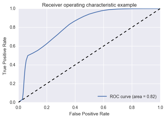
Training a Simple Logistic Regression Model

This example shows how to compute a logistic regression classifier and evaluate it’s performance using the receiver operating characteristic (ROC) curve.

>>> ds_train = ds_example3.split(0, [80, 20])
>>> ds_test = ds_example3.split(1, [80, 20])
>>> glm = analytics.generalized_logreg(['x1'], 'y', ds_train, affine=True, l1reg=0, l2reg=0.01).run()
>>> cc = analytics.roc(glm, ['x1'], 'y', ds_test, thresholds=32).run()

Plot the ROC and display the area under the ROC:

>>> plt.figure()
>>> plt.plot(cc.fpr, cc.tpr, label='ROC curve (area = %0.2f)' % cc.auc_roc)
>>> plt.plot([0, 1], [0, 1], 'k--')
>>> plt.xlabel('False Positive Rate')
>>> plt.ylabel('True Positive Rate')
>>> plt.title('Receiver operating characteristic example')
>>> plt.legend(loc="lower right")
>>> plt.show()

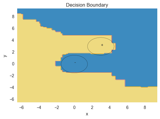
Training a Random Forest

In this example we train a random forest classifier on a binary classification problem associated to two overlapping gaussian distributions centered at (0,0) and (3,3). Points around (0,0) are labeled as in the negative class while points around (3,3) are labeled as in the positive class.

>>> ds_example4 = DataSet.from_table('tutorial.twoclass')
>>> rf = analytics.random_forest(['x1', 'x2'], 'y', ds_example4, 100, 1).run()

>>> plot_colors = "br"
>>> plot_step = 0.1
>>>
>>> x_min, x_max = 1.5-8, 1.5+8
>>> y_min, y_max = 1.5-8, 1.5+8
>>> xx, yy = np.meshgrid(
...     np.arange(x_min, x_max, plot_step),
...     np.arange(y_min, y_max, plot_step)
... )
>>> Z = rf.predict(np.c_[xx.ravel(), yy.ravel()])
>>> Z = Z.reshape(xx.shape)

Plot the decision boundary:

>>> fig, ax = plt.subplots()
>>> plt.contourf(xx, yy, Z, cmap=plt.cm.Paired)
>>> # Draw circles centered at the gaussian distributions
>>> ax.add_artist(plt.Circle((0,0), 1.5, color='k', fill=False))
>>> ax.add_artist(plt.Circle((3,3), 1.5, color='k', fill=False))
>>> ax.text(3, 3, '+')
>>> ax.text(0, 0, '-')
>>> plt.xlabel('x')
>>> plt.ylabel('y')
>>> plt.title('Decision Boundary')

This concludes the user tutorial section, so the connection should be closed.

>>> client.close()
>>> client.connected
False

Management and Administration

Administration tasks use the Client class from the leapyear module and admin classes from the leapyear.admin. These admin classes include:

• User

• Database

• Table

• Column

These classes provide API’s for various administrator tasks on the LeapYear system. All of the examples in the administrative examples section will require correct permissions.

Managing the LeapYear Server

Management requires sufficient privileges. The examples below assume the lyadmin user is an administrator of the LeapYear deployment system.

>>> client = Client(url, 'lyadmin', ROOT_PASSWORD)
>>> client.connected
True

User Management

User objects are used as the primary API for managing users. Below is an example of a user being created, their password updated, and finally their account is disabled.

>>> # Create the user
>>> user = User('new_user', password)
>>> client.create(user)
>>> 'new_user' in client.users
True
>>>
>>> # Update the user's password
>>> new_password = '{}100'.format(password)
>>> user.update(password=new_password)
<User new_user>
>>>
>>> # Disable the user
>>> user.enabled
True
>>>
>>> user.enabled = False
>>> user.enabled
False

Database Management

Database objects are used to view and manipulate databases on the server.

>>> # create database
>>> client.create(Database('sales'))
>>>
>>> # retrieve a reference to the database
>>> sales_database = client.databases['sales']
>>>
>>> # drop database
>>> client.drop(sales_database)

Table Management

Table objects are used to view and manipulate tables in a database on the server. Below is an example of how to define a data source (table) object on the LeapYear server.

>>> credentials = 'hdfs:///path/to/data.parquet'
>>>
>>> # create a table
>>> accounts = Database('accounts')
>>> table = Table('users', credentials=credentials, database=accounts)
>>>
>>> client.create(accounts)
>>> client.create(table)
>>>
>>> # retrieve a reference to the table
>>> users_table = accounts.tables['users']
>>>
>>> # drop a table
>>> client.drop(users_table)